Vertebrate brain theory

5.6        The directional selectivity of the visuel divergence grating

In the visual cortex V1 of vertebrates a directional selectivity of the so-called orientation columns is observed. These are groups of neurons that run through all six layers of the visual cortex and form small cylindrical columns. Their activity is selectively sensitive to the angle of inclination of a dark line against a light background. The neurons involved must therefore respond to dark objects, and are therefore of the dark on type.

We first analyze the response of a magnocellular ganglion cell of the retina of the dark-on type when a dark line is moved across its receptive field with a constant angle of attack from left to right. The line is moved quasi parallel to itself. We imagine the receptive field of the ganglion cell represented by a circle. Every dark object in the circle will cause an excitation of the ganglion cell.

For the recognition of bright lines on dark background the Hell-On-Ganglion cells are responsible (according to the author). We concentrate here on the dark on cells.

Let the line intersect the circle that represents the receptive field of the cell, so that part of the line becomes a tendon in the circle. The length of this chord will determine the rate of fire of the ganglion cell. We assume here that the excitation of the cell increases with the square of the chord length. Later we may be able to drop this assumption once we have understood the working principle of the orientation columns. At first we are only interested in the chord length.

Figure 58 - Chord length on the circle

The chord length will depend on the position of the straight lines, more precisely on the distance of the straight line from the center of the circle.

Figure 59 - Chord Length and Center Distance

A suitable variable for calculating the chord length is the distance of the chord from the centre of the circle. The known radius  forms the hypotenuse of a right-angled triangle whose cathets are h and half the chord length s/2. These three quantities are linked by the Pythagorean theorem.

Figure 60 - Calculating the chord length on a circle

So it's true:                     (Pythagoras)

This results in the following equation for the square of the chord length:

In general  apply, since r is the length of the hypotenuse of a right-angled triangle and h is the length of a cathetus. Otherwise, the square of the chord length becomes negative, i.e. the chord length becomes an imaginary number. Then the straight line no longer intersects the circle, the formula becomes inapplicable.

We assume here that the rate of fire f of the ganglion cell, in whose receptive field the tendon of length s darkens the visual field, increases quadratically with the tendon length:

We now consider the chord length or its square using a coordinate system where the receptive field is not in the coordinate origin. The center of the circle K, which should represent the receptive field of the ganglion cell, should be the point P_k in the coordinate system, to which we assign the coordinates x_m and y_m. Then we can also represent the point P_k as P_k(x_m; y_m).

The line g, which may intersect the circle K, has the angle φ to the x axis. Its distance from the coordinate origin P(0;0) is r.

The circle center P_k(x_m; y_m) may be at a distance r_k from the coordinate origin P(0; 0). The line connecting the two points has the length r_k and should form the angle φ_k with the x-axis..

Then the following equation applies to the chord length s_k 

                                          (4.2.1)

The Pythagorean theorem and the representations of the quantities x_m, y_m over the sine and cosine of the angle difference. Useful is the graphic representation of the connections necessary for the derivation in the following figure.

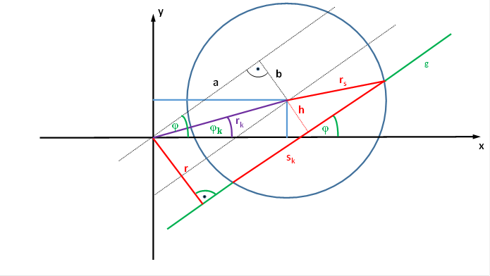Figure 61 - Chord length calculation for a shifted receptive field

With reference to the above figure: 

We assume that a dark on ganglion magnocellular cell, whose receptive field is intersected by a straight line with the angle of rise φ and the distance r from the coordinate origin, has a fire rate f_k, which is a function of φ and r.

    (4.2.2)

We now investigate the firing rates f12, f2, f3 and f4 of four retinal ganglion cells of the described type under the assumption that they are arranged in the Cartesian coordinate system exactly along the coordinate axes and have a distance r = 1 from the coordinate origin. This is sketched in the following figure.

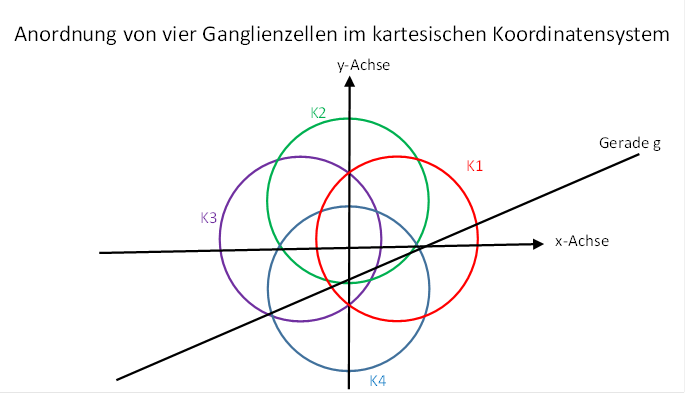
Figure 62 - Arrangement of four visual ganglion cells

Each of the four ganglion cells has a circular receptive field with radius r_s. The partial or complete overlapping of the four receptive fields is important. The straight line has again the angle of ascent φ.

The following special features apply to this arrangement of ganglion cells:

                                   

This simplifies the formulas for the rate of fire 

 of the associated retinal ganglion cells:

                                  (4.2.3)

                                (4.2.4)

                                  (4.2.5)

                                 (4.2.6)

These four fire rates travel from the retina via the Corpus geniculatum laterale to the visual cortex or visual cranial turning loop from which it emerged. All following considerations now refer to the signal propagation of these four input signals in the visual cortex. The topological arrangement of the four input signals should be preserved. Therefore there are four input neurons in the visual cortex, which in turn form the corners of a square and whose fire rates are the values f₁, f₂, f₃ and f₄ according to our formulas.

We fill the square area with output neurons, which get their excitation via interneurons from the four input neurons. Simplified, we can divide the square by equally spaced horizontal and vertical grid lines, in whose intersections the output neurons may be located.

We select any output neuron and calculate its excitation. This is made up of four parts, because it receives an excitation part from each of the four input neurons. However, a distance-dependent damping occurs, for which we assume a quadratic influence of the distance. The rate of fire of the considered output neuron therefore satisfies the equation 

                                                                         (4.2.7)

The fire rates f_k originate from the described retinal ganglion cells.

We can also derive suitable formulas for the distances r₁, r₂, r₃  and r₄ of the output neuron to the four input neurons. For this we need the following figure.

We note that the input neurons lie on the coordinate axes according to our specifications and have the distance 1 from the coordinate origin.

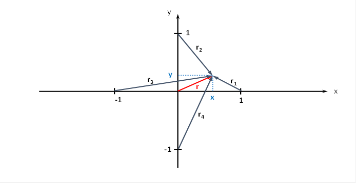
Figure 63- Radius vectors to a neuron at point P(x,y)

At the latest here it becomes clear that in this case, too, we are dealing with a plane divergence grating, for whose excitation function we have already derived the formula (3.6)

                (4.2.8)

In this equation we still have to insert the derived formulas for the fire rates delivered by the retinal ganglion cells of the dark-on type when a dark line with a rising angle φ is sighted.

If there is an inclined straight line in the field of vision of the four retinal ganglion cells, we can insert the calculated fire rates into this equation and obtain for the total excitation f of the considered output neuron the equation

       

        (4.2.9)

We recapitulate the most important requirements: The output neuron in the point  is immovable. It cannot move actively. Therefore the parameters and  constant and unchangeable.

Furthermore, we assume that the angle of rise φ of the straight line, which also overlaps the receptive fields of the four retinal ganglion cells, also remains constant.

If now the line is shifted parallel to itself, only its distance r from the coordinate origin changes. In this case it is observed in the experiment that the output neuron fires at maximum exactly when the angle of rise of the straight line takes on a very specific value. Neighboring output cells show a higher rate of fire, but at different angles.

Mathematically, this means that the fire rate f of the output cell under consideration in the point is a function of the distance r and has a maximum. This means that the first derivative from f to r must be zero, while the second derivative to r should be negative and non-zero. Precisely then the excitation function f would have a maximum. We therefore calculate the first and second derivatives to r. Here we note that all quantities except r represent constants. We set the first derivative to zero.

(4.2.10)

The second derivative after r gives the simple equation

                                                                                     (4.2.11)

Thus the second derivative fulfils the condition for the existence of a maximum, it is really negative less than zero.

The equation resulting from zeroing the first derivative after r is first simplified by using the common factor 

 

divide. This is allowed because this factor is not equal to zero. So we get the first simplification:

(4.2.12)

The conversion into the representation with hyperbolic functions is advantageous. 

Using these relations we get the condition

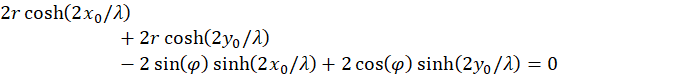
                                                                                                                                  (4.2.13)

Thus we have a condition for the existence of a maximum of the excitation function f of the output neuron in the point received:

                                                                                                                                  (4.2.14)

This equation of determination can be solved by the angle φ. For this we use the formula

With

we obtain the equation 

                                                                                                                                  (4.2.15)

This can be transformed into

                                                                                                                      (4.2.16)

Taking into account   finally results in the equation for the angle φ, where the output neuron is located at  is assuming its maximum rate of fire f:

                                                                                                                      (4.2.17)

                                                        (4.2.18)

For this value of φ the derivative of the rate of fire f to r is zero, the second derivative being less than zero. Thus f assumes a local maximum. Thus, if the inclined line separating the receptive fields of the four retinal ganglion cells involved has this angle of rise φ and the distance r from the coordinate origin, the output neuron fires in the visual cortex with the coordinat  and has a local maximum. It is precisely this behavior that characterizes the neurons of the orientation columns in the visual cortex. It is not based on learning processes, but on the propagation of excitation of neighbouring magnocellular ganglion cells in the visual cortex, whereby this propagation is subject to a distance-dependent attenuation. In our model we postulated the quadratic dependence of the rate of fire of the ganglion cells on the length of the tendon, as well as the quadratic exponential damping. This model led directly to an equation for determining the optimal angle at which the strongest firing of the output neuron occurs. Other assumptions will lead to analogous results.

We now use the possibility to represent the equation of determination as a function of x and y. Then, for example, we can display the relationship between the best angle and the location of an output neuron in Excel.

First of all, the constant part in the diagram is  of the second summand is displayed graphically:

Figure 64 - The Angle Dependence of the Term T2

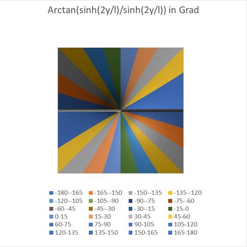The displayed angle was assigned a different color at intervals of 15 degrees (see legend in the diagram).

This shows the contribution of the second summand in the equation of determination for φ. This contribution is independent of the distance r of the straight line to the coordinate origin.

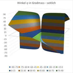
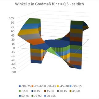
The following two diagrams show the angle φ of the total formula (18.5.3.21) as a function of the values x and y. In the left-hand diagram seen from the side and next to it from above. First we choose the value r = 0.

Figure 65 - Display of the angle seen from the side

igure 66 - Viewing the angle from above

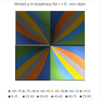
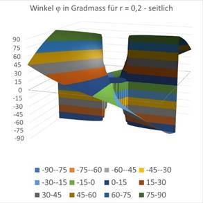
The influence of the radius r can also be displayed graphically. In the above illustration r = 0 was given. The figures are Excel graphics, where the derived formulas for the angle φ were used to create the diagram. For a value of r = 0.2 the following graphs are obtained.

Figure 67 - The influence of r on the directional selectivity

Figure 68 - The influence of r

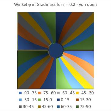
Here you can see that a circle-like small area of the coordinate origin responds to the angle φ = 0, while in the rest of the area the angles are arranged like a windmill, with each angle interval being assigned a different color in steps of 15 degrees. Exactly this was also done in the experiments on the angular selectivity of the orientation columns in the visual cortex V1. In this monograph, the mathematical context was presented for the first time.

Finally the graphics for r = 0.5.

Figure 69 - Orientation Columns for Large r

Figure 70 - Orientation columns with large r

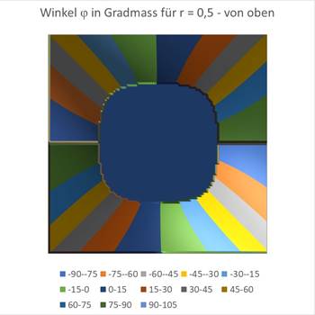
You can see that the circle around the coordinate origin, in which there is a maximum at an angle of incidence of 0 degrees, becomes larger as r grows. Approximately at the value of r = 0.7, the blue area is already so large that it fills almost the entire square. At about this value, the retinal ganglion cells no longer react with meaningful output because the inclined straight line no longer darkens the receptive fields sufficiently.

The blue circle at the origin of the coordinates, to which the tilt angle  but does not represent the area where the output neurons fire most strongly at an angle of 0 degrees. Rather, the function value of the angle is not defined at this point. Only Microsoft's Excel program replaces the undefined angle value with the numerical value 0, because it uses the

calculable angle values - this is what the programmers from Excel decided. This solution is far better than issuing hundreds of error messages that would read: "Function value not defined!

herefore we have to prove at this point why the function values are not defined in the "circle" shown in blue. Equation (4.2.18) contains the term .

The function arcsin(x) is only defined for x-values in the interval from -1 to +1. If x is outside this interval, there is no real value of this function arcsin(x). Excel then outputs - simplified - the value zero, because error messages at this point would confuse the user.

An increase in the value of the parameter r in the term  results in the function's argument for certain parameter values being outside the allowed interval. The greater r becomes, the greater the number of invalid values.

The cause is simple: the length of the tendon must not be negative. If the inclined line no longer intersects the circle, there is no chord length and the formula leaves the permissible range.

To sum up, one could say

Theorem of the directional selectivity of orientation columns in the visual cortex

The directional selectivity of the orientation columns in the primary visual cortex and their mode of operation are based on signal propagation in plane divergence grids with distance-dependent, exponential signal attenuation. This signal divergence primarily increases the redundancy and thus the reliability of the system. Directional selectivity is the result of signal propagation on non-markless fibers where exponential attenuation occurs. The latter causes the directional selectivity.

By the way, this directional selectivity is independent of any movement - especially a parallel shift of the inclined line. Only the center distance r of the line to the coordinate origin enters the formulas, the angle of attack φ is constant. And it has been shown that for each angle of attack a different population of neurons fires at most, and these populations for different angles of attack are arranged around the center like a windmill, as can be seen in the diagrams.

The special feature is that a flat divergence grating does not require any learning processes, its operating principles are present from the very beginning. Thus, the assumption that in the primary cortex fields - which do not receive their input from the spinocerebellum - learning neural networks are present proves to be unnecessary. The directional selectivity is not learned, it is present from the very beginning. It is based on elementary laws of nature, in particular the exponential damping of excitations when propagating in the surface.

This explains why nest prey are immediately able to detect objects. Objects are first recognized by the perception of their contours, which are detected as oriented line elements by the orientation columns in the cortex.

If the distance-dependent damping is not caused by an exponential function, but by another class of functions that is also convex, analogous results are obtained. In this respect, the function known as the cable equation can also be replaced by other functions.