Vertebrate brain theory

         

2          

3          

         

5          

We now analyze the functioning of plane divergence grids using the example of one with four input neurons. Divergence grids with two input neurons have already been analyzed. The starting point was the cable equation for non-markless axons, which is reproduced again here.

The cable equation for non-markless axons describes the decrease in excitation along an axon, where E0 is the initial excitation at the start of the axon and E is the excitation value measured at distance x from the start of the axon:

            .                                             

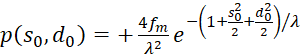
  The quantity λ  is called the longitudinal constant of the neuron.

The excitation function can be shown graphically in a diagram, where the decrease in excitation can be clearly seen as the distance increases.

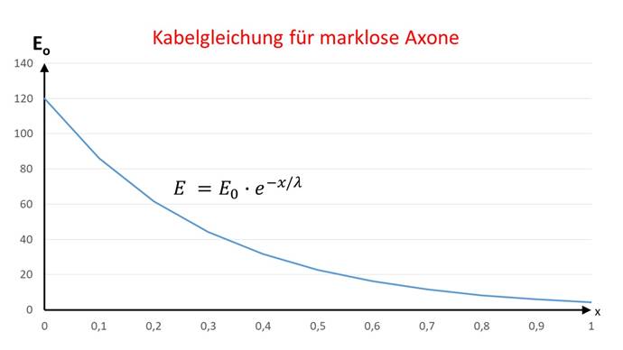
Figure 44 - Cable equation for non-markless fibers

From the cable equation for non-markless fibers, the fire rate f can be inferred directly. This fire rate f has a neuron that is at a distance x from an input neuron with the fire rate f0 and is connected to it via a non-markless axon. Here, the excitation E is replaced by the fire rate f.

           

The graphic representation of the fire rate function as a function of distance x is shown in the following figure.

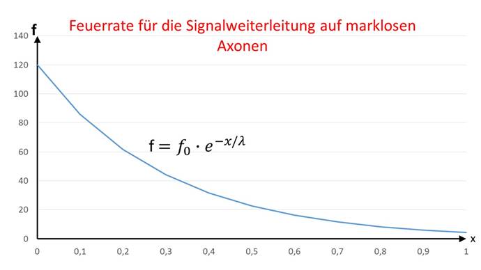
Figure  45 - Fire rate for signal propagation on non-markless fibers

The excitations of two neurons overlapped in a linear divergence grid. In a plane divergence lattice, the excitation is propagated in the area in which both the input neurons and the output neurons are distributed.

We compare both divergence grids in the following figure, which has already been used.

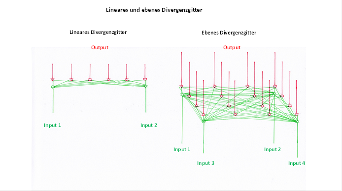
Figure  46 - Linear and plane divergence grating in comparison

The plane divergence lattice may have four input neurons. We arrange the four input neurons in a coordinate system in such a way that they lie on the coordinate axes at a distance of 1 from the zero point, as the following figure shows.

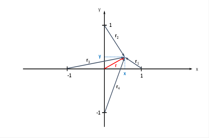
Figure  47 - Planar divergence grid with four input neurons

At the point P with the coordinates P = (x ; y), to which the radius vector r belongs, there may be - representative for the many hundreds of output neurons - one output neuron, whose excitation we want to calculate.

We are interested in the excitation of those neurons that are located in the square with side length 2, whose center is located in the coordinate origin. Each of the output neurons located there is synaptically linked to the four input neurons, as shown in the above figure on the plane divergence lattice. We are especially interested in the extreme values of the excitations in this square, i.e. minima and maxima. For this we have to do some mathematical considerations.

The following equations are obtained for the radius vectors r1 to r4 using the Pythagorean theorem:

                                     (3.1)

 

                                     (3.2)

 

                                     (3.3)

 

                                     (3.4)

 

While in the linear divergence lattice the exponential damping increased with distance, we assume a square exponential dampingin the plane divergence lattice, because the excitation of the input neurons must not propagate along a straight line, but within a surface.

Are the four input neurons located in the points , ,  and and receive the excitations with the fire rates f1, f2, f3 and f4, then under our conditions the fire rate f of the output neuron can be determined in the point  be calculated as a total:

.                                  (3.5)

If the relations (3.1) to (3.4) are used for the four radius vectors r1 to r4 and the common factors are summarized, the following results are obtained:

 

         (3.6)

 
Here x and y are the coordinates of the output neuron at point P(x,y) in the Cartesian coordinate system.

We assume that the excitations f1 to f4 are supplied by four receptors. Two of them must be complementary to each other in the divergence lattice, i.e. they must be separated by signal inversion. These might be the signals of two muscles working against each other. We choose f1 and f3 as the first pair of complementary signals that are delivered by the receptors _R1 and _R3.

For these two receptor signals we choose the exponential approach according to

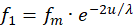                                 (3.7)

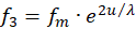                                   (3.8)

Here the original size u could correspond to the joint angle, for example.

Neurologists will (justifiably) object that an exponential characteristic is not generally accepted. Many assume that the relationship between a primal quantity and the rate of fire of the perceptual receptors is logarithmic. However, in this monograph we refer (initially) to the motor area. It seems unrealistic to assume that muscle traction must quadruple in order to double the rate of fire of e.g. the muscle spindles. This also means that the muscle traction force must increase by a factor of 25 for the rate of fire to increase fivefold. Or the muscle traction must be increased by a factor of 100 so that the rate of fire increases by a factor of 10. Such pulling forces on muscles are unrealistic and would lead to their destruction.

We choose the exponential approach. This is much more realistic.

In other areas, for example in the visual field, control mechanisms are used which produce a logarithmic characteristic curve. Here, the light intensity can be regulated by the narrowing of the pupil, and there is also a regulated inhibitory effect among the visual receptors, for example by the amacrine cells, which increases with brightness.

We select for the greatness u the joint angle, the measured value of which is transformed by the responsible receptor (e.g. the tendon organ) into a fire rate with an exponential sensitivity curve. The quantity fm represents the mean rate of fire. It is supplied by the receptor if the original quantity u lies exactly in the middle of the associated measurement interval <u1; _u2>.

And since each joint has two muscles working against each other, the two fire rates f1 and f3 are the result, and are inverse to each other.

The firing rate f1 is strictly monotonically decreasing, i.e. of the off-type. The firing rate f3, on the other hand, is strictly monotonically increasing and therefore of the on-type. For a neuronal signal evaluation, both firing rates and thus both receptors are always required.

Analogously, for the two remaining firing rates f2 and f4 there may also be two receptors _R2 and _R4, which likewise transfer the value of another greatness v into two complementary firing rates, the mean firing rate being the same.

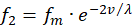                      (3.9)

                        (3.10)

Again, one rate of fire is strictly monotonically falling and the other rising.

In the plane divergence grating, the original quantities u and v are included in the exponents of the fire rate with the factor 2, since we have also assumed a quadratic consideration of the distance in the excitation function. Therefore, the receptors must also provide a stronger input so that the receptor neurons in the plane divergence lattice receive a useful excitation at all, because this excitation must spread over the surface. The neurons that transmit this excitation in the plane divergence lattice are also stronger and larger.

In these fire rates, the quantities u and v represent the strength of measured primal quantities supplied by the four receptors. But why do we assign f1 to f3 and f2 to f4 and not f1 to f2 and f3 to f4? Because we choose the arrangement as it is found in a joint with two degrees of freedom. While f1 is assigned to the flexor and f3 to the extensor for one degree of freedom, f2 and f4 are responsible for the second degree of freedom. Therefore, the arrangement of the associated muscles and tendons at the joint would be the same as we have chosen for the assigned fire rates.

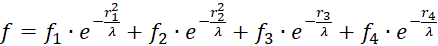
If we apply the above fire rates (3.7) to (3.10) to equation (3.6), the excitation of an output neuron at point P(x,y) results in the functional equation

            (3.11)

 

The use of the hyperbolic function

                     (3.12)

 

provides the simplification

     (3.13)

Now we can analyze the effects of changes in the quantities u and v measured by the receptors R₁ to R₄ on the excitation of an output neuron.  

In the linear divergence grating, the excitation function had a minimum, which ultimately encoded the strength of the measured original quantity. What about the excitation function in the plane divergence grating? Is there any significant difference?

This question must be answered in the affirmative. In the plane divergence lattice, the strength of the original quantities is not encoded by an excitation minimum, but by an excitation maximum. The excitation function (3.11) or (3.13) has an excitation maximum near the point P(u,v).

Theorem of maximum coding of the great magnitudes in the plane divergence lattice with four input neurons

Let u be a primal quantity whose value is transformed by means of two complementary receptors _R1 and _R3 into two complementary firing rates f1 and f3 according to  

and 

.

Let v be a further independent original quantity, the value of which is transformed by means of two complementary receptors _R2 and _R4 into the complementary fire rates f2 and f4 according to

 

and

.

 

A plane divergence grating receives - with reference to a Cartesian coordinate system - the four firing rates in a well-ordered manner in such a way that f1 at point P(1,0), f2 at point P(0,1), f3 at point P(-1,0) and finally f4 at point P(0,-1) becomes effective as input.

Then the excitation function f(x,y) has the form

                         (3.14)

                         (3.15)

 

For each point P(xo, _yo), equations (3.14) and (3.15) can be used to calculate what value the original quantities u and v must have so that the neuronal excitation at this point assumes its maximum.

A small restriction for u and v results from the fact that the function artanh(x) is not defined for all x. From a neurological point of view, we are only interested in the maxima within the square with side length 2, whose center is formed by the coordinate origin and in which the output neurons are located.

To derive the conditions (3.14) and (3.15) we have to put the function (3.13) into a more convenient form.

      (3.16)

 

Here s = x + y and d = x - y, i.e.

and

.

 

It follows from this

                                                                       (3.17)

 

Thus (3.16) becomes

      (3.18)

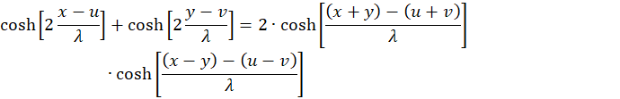
Now we reshape the expression with the hyperbolic functions.

Because of

                                      (3.19)

applies

We set u + v = w and u - v = z and because of x + y = s and x - y = d we get the equation

     (3.20)

Thus (3.13) receives a new representation:

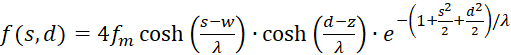                   (3.21)

 

This representation is easier to handle when differentiating, since the variables s and d appear in separate factors.

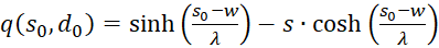
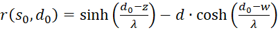
For the determination of extreme values we calculate the first derivative of both s and d.

     (3.21)

 

     (3.22)

 

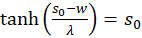
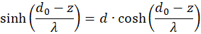
The derivatives to s and to d must be zero, so that an extreme value can exist at all (necessary conditions). Since the mean rate of fire fm and λ are greater than zero, the exponential expression is generally greater than zero and the function cosh(x) is greater than 1, the last factor in the brackets must be zero. Thus we obtain two conditional equations for the values s_o and d_o, in which an extreme value could exist.

     

 

and

           (3.23)

.                                                

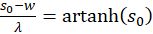
Forming results:

                               and                         (3.24)

                          and                      (3.25)

                    and              (3.26)

 

Because of u + v = w as well as u - v = z and x + y = s and x - y = d the following results

                                                       (3.27)

                                                       (3.28)

Addition of both equations yields

                          (3.29)

                          (3.30)

We express x and y by polar coordinates and consider Figure 49. Then we have

Inserting into the above equation and applying addition theorems for trigonometric functions provides:

                                     (3.31)

                                     (3.32)

with

.                                                                                       (3.33)

Then it's on:

    (3.34)

    (3.35)

 

Since the function f(x) = artanh(x) is only defined for x values with -1 ≤ x ≤ +1, i.e.

 

there are two conditions for the sizes r and α.

This means:

For the radius vector r this means the following condition for the existence of an extreme value:          

                                                                                (3.36)

 

The application of the following addition theorem to (3.29) and 3.30 is appropriate:

and returns the extreme value condition

                                                            (3.37)

 

                                                            (3.38)

 

If, on the other hand, the representation in polar coordinates according to (3.31) and (3.32) is used, the result is an extreme value condition:

                              (3.39)

                          (3.40)

 

The equations (3.36) and (3.37) or (3.38) and (3.32) as well as (3.39) and (3.40) must be fulfilled so that the excitation function (3.13) has an extreme value in point (xo, _yo). They do not allow the determination of x and y, but for any value of x and y from the definition range the required values for the original quantities u and v can be determined, so that an extreme value can be present there.

However, for this to happen, the sufficient conditions for the existence of extreme values must also be fulfilled.

We remember:

If at the position _so and _do fs(_so, _do) = 0 and fd(_so, _do) = 0 and the inequality

,                                        (3.41)

then a minimum is present at this point if is and a maximum when is.

We will proceed in several steps.

(1)   First, we prove that is.

(2)   Then we show analogously that also is.

This makes the product  .

(3)   Further we show that is. This would prove the inequality 3.41. And since the second derivative after s is negative, it would be proved that there is a maximum.

First of all we prove (1).

 

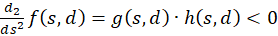
For this purpose, we calculate the second derivative, which we write as the product of two factors for better clarity:

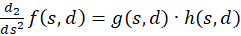                                                             (3.42)

 

with

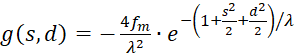
                                (3.43)

                  (3.44)

 

The factor g(s,d) is generally negative for all values of s, d and w.

We therefore only check whether the factor h(s,d) in the point P(_so, _do) is positive, because then the product of both would be negative and one of two sufficient conditions for the existence of a maximum would be fulfilled. For this we remember the equation (3.23):

Switching delivers

We use this in equation (3.44) and consider x = xo and y = y_o:

  (3.45)

Let's recap:

     (3.46)  

                                     

Taking 1 λ > into account, the inequality for any value is

 

and consequently

                                                                  (3.47)

 

Thus the second derivative after s is less than zero, so that (1) would be proved.

Now we show (2).

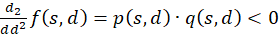                                                                 (3.48)

 

with

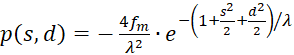
                                (3.49)

            (3.50)

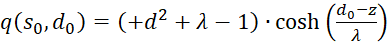
The first factor is negative again. The second is positive because we can substitute. According to (3.23)

 

We're remodeling:

Inserting in (3.50) gives for s = s_o and d = d_o

  (3.51)

Summarising provides

                                  (3.52)

 

Because of λ > 1, the following now applies in general

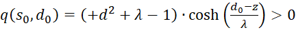                             (3.53)

Since p(s,d) was less than zero and q(s,d) greater than zero, the product of both is negative.

Thus the equation for the second derivative after d is also

                                                                 (3.54)

The Equation

                                           (3.55)

would always be fulfilled if the following could be proven:

                                                                                         (3.56)

We calculate this mixed derivative and present it as the product of three factors:

                                           (3.57)

The following applies

                                                 (3.58)

                                       (3.59)

                                        (3.60)

 

 

                                      

The factors and  are zero, as already shown in (3.23). Thus the mixed derivative is also equal to zero. Thus our excitation function has a maximum at the derived coordinates. This proves the theorem of maximum coding in the plane divergence lattice with four input neurons.

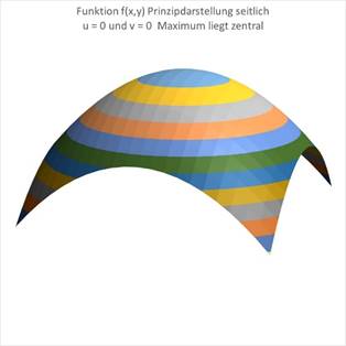
For the following observations we choose again the representation of the excitation function in the variables x and y.

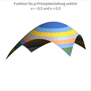
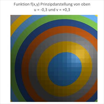
We can now get an idea of what the two-dimensional excitation function f(x,y) looks like and that it actually has a maximum at the corresponding point close to the point P(u,v).

 

Figure  48 Principle representation No. 1 Excitation function

Figure  49- Principle diagram no. 2 Excitation function

 

Figure  50- Principle representation no. 3 Excitation function

Figure  51- Principle diagram no. 4 Excitation function

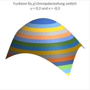
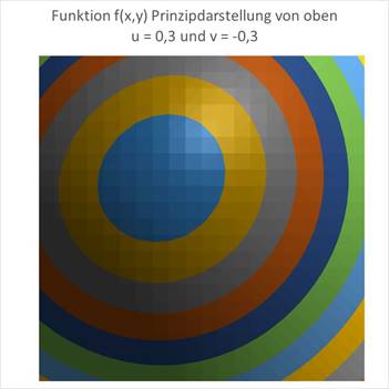
For u = 0.3 and v = -0.3 the maximum moves to the left and back:

For u = -0.3 and v = +0.3 the maximum moves to the right and forward:

 

Figure  52- Principle representation no. 5 Excitation function

Figure  53- Principle representation no. 6 Excitation function

 

Lateral inhibition often occurs in plane divergence grids. Strongly excited neurons inhibit less excited ones via interconnected inhibitory interneurons. Thus, excitation is retained in the area surrounding the location of maximum excitation, while it is completely inhibited in the rest of the square divergence lattice. This creates the impression of a strongly excited population of neurons, which migrates around in the plane divergence lattice when the magnitudes u and v change. Periodic movements result in the Lissajous figuresmentioned above.  

Theorem of extreme value selection in plane divergence grids

Strong lateral inhibition in plane divergence grids with maximum coding causes an active neuron population to be observed only around the point of maximum.

The signal divergence first occurred in the nucleus olivaris. There, the input of complementary signals was transformed into minimum-coded signals, which were then inverted in the cerebellar nucleus so that they were again maximum-coded.

Signal divergence in the plane divergence grating with maximum coding results directly in maximum coded signals. A signal inversion, as occurred in the cerebellar nucleus, would again produce useless minimum coded signals. Therefore the nucleus olivaris was unusable for such flat divergence grids.

Level divergence grids therefore had to be created elsewhere in the brain, even if they were not primarily designed for maximum coding of signals at all. The main advantage of plane divergence gratings was initially the increase in reliability. Signals were transmitted redundantly to groups of neurons, each of which formed a plane divergence grating. If individual neurons failed, the target structures still received their input.

The fact that exponential signal attenuation resulted in a maximum coding of the strength of the original magnitudes was - like everything in evolution - not planned, but rather the random consequence of the action of natural laws in the propagation of action potentials on non-markless axons.

It must be pointed out here that the derived maximum coding only occurs because in a joint with several degrees of freedom the muscle tension receptors of the muscles are coupled together for the different planes of movement. In the case of non-coupled variables, flat divergence grids can also deliver minimum-coded signals. In general, extreme value-coded signals occur here. In the visual field, there is a minimum coding for color vision, but a maximum coding for shape vision. This will be shown in further chapters.

Of course, the question arises whether plane divergence grids actually exist in the vertebrate brain?

Such divergence grids can only be found in neuron areas that belong to the grey matter, because the axons that divergently transmit excitation must be non-markless. This means that they must not have myelin sheaths that are typical for the white matter. All nuclei of the grey matter and the cortex cortex are therefore eligible. Furthermore, the number of output neurons must clearly exceed that of input neurons. Thus, many neuron nuclei are excreted. Finally, a maximum coding must be detected in these neuron areas. Thus, the nucleus olivaris is eliminated completely and almost only the cortex remains. However, the nuclei of the grey matter in the limbic system, especially the amygdala,should not be forgotten. And in birds and reptiles there is the DVR and in birds the hyperpallium.

A further problem is the existence of convergence gridswhich work exactly inversely to the divergence grids and have the same structure in principle, only that input and output are swapped. Therefore, convergence grids have significantly fewer output neurons than input neurons - an important differentiating feature.

In mammals, one finds convergence grids in the cortex.

Theorem of the existence of plane divergence grids in the cortex

Those primary cortex regionsthat receive their receptor input via thalamic nuclei and not via the cerebellum consist of flat divergence grids. The topology of the sensory body models remains in these cortex areas despite the signal divergence.

This leads to the next question: What evidence is there for the work of plane divergence grids in the primary cortex regions? The following chapter is devoted to this question.

Before we do this, we need to understand how plane convergence grids work.